Introductory demo

This document is a functional Jupyter notebook showing how to work with OSIRIS using the duat Python interface. You can also use it with python scripts or from the interpreter, but the notebook is a handy way to use the package I suggest you to consider.

The updated version of this notebook can be download here.

First, import some modules.

import os
import numpy as np
import matplotlib.pyplot as plt

from duat import config, plot, run

/usr/lib/python3.6/site-packages/h5py/__init__.py:36: FutureWarning: Conversion of the second argument of issubdtype from `float` to `np.floating` is deprecated. In future, it will be treated as `np.float64 == np.dtype(float).type`.
  from ._conv import register_converters as _register_converters

If a warning on not found executables was raised for you, add some code setting the path to the folder with the executables: run.set_osiris_path(path.join("path", "to", "osiris", "folder"))

Creating a simulation

The config module offers functionality to create a simulation.

# Create a config file with the defaults
sim = config.ConfigFile(1)  # Argument -> dimension
# Check the generated code
print(sim)

node_conf
{
  node_number(1:1) = 1,
  if_periodic(1:1) = .true.,
}

grid
{
  coordinates = "cartesian",
  nx_p(1:1) = 1024,
}

time_step
{
  dt = 0.07,
  ndump = 10,
}

space
{
  xmin(1:1) = 0,
  xmax(1:1) = 102.4,
  if_move(1:1) = .false.,
}

time
{
  tmin = 0,
  tmax = 7,
}

emf_bound
{
  type(1:2, 1) = 0, 0,

}

particles
{
  num_species = 2,
  num_cathode = 0,
  num_neutral = 0,
  num_neutral_mov_ions = 0,
}

!---Species configuration
!---Configuration for species 1
species
{
  num_par_max = 2048,
  rqm = -1,
  num_par_x(1:1) = 2,
  vth(1:3) = 0, 0, 0,
  vfl(1:3) = 0, 0, 0,
}

profile
{
  fx(1:6, 1) = 1, 1, 1, 1, 1, 1,

  x(1:6, 1) = 0, 0.9999, 1, 2, 2.001, 10000,

}

spe_bound
{
  type(1:2, 1) = 0, 0,

}

diag_species
{
}


!---Configuration for species 2
species
{
  num_par_max = 2048,
  rqm = -1,
  num_par_x(1:1) = 2,
  vth(1:3) = 0, 0, 0,
  vfl(1:3) = 0, 0, 0,
}

profile
{
  fx(1:6, 1) = 1, 1, 1, 1, 1, 1,

  x(1:6, 1) = 0, 0.9999, 1, 2, 2.001, 10000,

}

spe_bound
{
  type(1:2, 1) = 0, 0,

}

diag_species
{
}

# Let's change some parameters:
# Parameters can be edited using the python item access notation
sim["time"]["tmax"] = 30.0
# Beware the python indexes starting at zero. E.g., "1" is the second particle species
sim["species_list"][0]["species"]["vfl"] = [0.0, 0.0, 0.6]
sim["species_list"][0]["species"]["num_par_x"] = [200]
sim["species_list"][1]["species"]["vfl"] = [0.0, 0.0, -0.6]
sim["species_list"][1]["species"]["num_par_x"] = [200]

# Order of output is handled by duat. We can now change parameters that will appear before in the generated file
sim["species_list"][0]["diag_species"].set_pars(ndump_fac=1, reports="ene")

# We can benefit from python preprocessing power
ene_bins = np.arange(0, 0.5, 0.02)
sim["species_list"][1]["diag_species"].set_pars(ndump_fac=1, ndump_fac_pha=1, pha_ene_bin="x1_|charge|",
                                                ene_bins=ene_bins, n_ene_bins=len(ene_bins))

# Even if a section was not created before, accessing it with the index notation will create it
sim["diag_emf"]["reports"] = ["e1", "e2", "e3"]
sim["diag_emf"]["ndump_fac"] = 5

# This also works with lists
sim["zpulse_list"][0].set_pars(a0=1.0, omega0=1.0, phase=0.0, pol_type=1, pol=0, propagation="forward",
                               lon_type="gaussian", lon_x0=40, lon_range=20, lon_duration=50, per_type="plane")

# Check the generated code again
print(sim)

node_conf
{
  node_number(1:1) = 1,
  if_periodic(1:1) = .true.,
}

grid
{
  coordinates = "cartesian",
  nx_p(1:1) = 1024,
}

time_step
{
  dt = 0.07,
  ndump = 10,
}

space
{
  xmin(1:1) = 0,
  xmax(1:1) = 102.4,
  if_move(1:1) = .false.,
}

time
{
  tmin = 0,
  tmax = 30,
}

emf_bound
{
  type(1:2, 1) = 0, 0,

}

diag_emf
{
  reports(1:3) = "e1", "e2", "e3",
  ndump_fac = 5,
}

particles
{
  num_species = 2,
  num_cathode = 0,
  num_neutral = 0,
  num_neutral_mov_ions = 0,
}

!---Species configuration
!---Configuration for species 1
species
{
  num_par_max = 2048,
  rqm = -1,
  num_par_x(1:1) = 200,
  vth(1:3) = 0, 0, 0,
  vfl(1:3) = 0, 0, 0.6,
}

profile
{
  fx(1:6, 1) = 1, 1, 1, 1, 1, 1,

  x(1:6, 1) = 0, 0.9999, 1, 2, 2.001, 10000,

}

spe_bound
{
  type(1:2, 1) = 0, 0,

}

diag_species
{
  ndump_fac = 1,
  reports = "ene",
}


!---Configuration for species 2
species
{
  num_par_max = 2048,
  rqm = -1,
  num_par_x(1:1) = 200,
  vth(1:3) = 0, 0, 0,
  vfl(1:3) = 0, 0, -0.6,
}

profile
{
  fx(1:6, 1) = 1, 1, 1, 1, 1, 1,

  x(1:6, 1) = 0, 0.9999, 1, 2, 2.001, 10000,

}

spe_bound
{
  type(1:2, 1) = 0, 0,

}

diag_species
{
  ndump_fac = 1,
  ndump_fac_pha = 1,
  pha_ene_bin = "x1_|charge|",
  ene_bins(1:25) = 0, 0.02, 0.04, 0.06, 0.08, 0.1, 0.12, 0.14, 0.16, 0.18, 0.2, 0.22, 0.24, 0.26, 0.28, 0.3, 0.32, 0.34, 0.36, 0.38, 0.4, 0.42, 0.44, 0.46, 0.48,
  n_ene_bins = 25,
}



!---zpulse_list
zpulse
{
  a0 = 1,
  omega0 = 1,
  phase = 0,
  pol_type = 1,
  pol = 0,
  propagation = "forward",
  lon_type = "gaussian",
  lon_x0 = 40,
  lon_range = 20,
  lon_duration = 50,
  per_type = "plane",
}

Running a simulation

The config module offers functionality to create a simulation

# A directory for the run
run_dir = os.path.join(os.path.expanduser("~"), "test-run")

# Run the simulation. This also checks for errors, but note they are not always detected
myrun = run.run_config(sim, run_dir, clean_dir=True)

# The created run instance offers some information of the run in progress.
myrun

Run<test-run [RUNNING (160/429)]>

# Other methods are available in the Run object. See the documentation for more information.
print("Size in disk of the run: %.2f MiB" % (myrun.get_size()/1024/1024))

Size in disk of the run: 3.78 MiB

Plotting the results

The plot module offers functionality to create a simulation

# Diagnostic objects can be used even if the run is in progress
diagnostics = myrun.get_diagnostic_list()
for d in diagnostics:
    print(d)

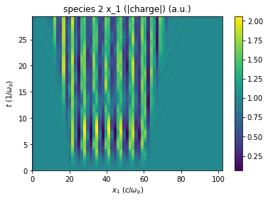
Diagnostic<species 2 x_1 (|charge|) ([64], 26, 43)>
Diagnostic<E_2 ([1024], 1, 9)>
Diagnostic<E_1 ([1024], 1, 9)>
Diagnostic<E_3 ([1024], 1, 9)>
Diagnostic<Kinetic Energy ([1024], 1, 43)>

# Methods like time_1d_colormap allow to represent a map
fig, ax = diagnostics[0].time_1d_colormap(dataset_selector=np.sum)
# The returned Figure and Axes instances allow for customization and export.
# Note the method itself takes a parameter for automatic exportation

# The time_1d_animation method allows to visualize a function in time
fig, ax, anim = diagnostics[2].time_1d_animation()
# This can be exported using the anim object or given a parameter to the function.

# In Jupyter you can plot this with:
from IPython.display import HTML
HTML(anim.to_html5_video())
# mpeg must be installed for this to work!
# The video can be downloaded from the output.

# Do the same as a color map
fig, ax = diagnostics[0].time_1d_colormap(axes_selector=(np.sum,))

# For manual manipulation use the get_generator method
gen = diagnostics[1].get_generator()
# This returns a generator that provides data when iterated
for snapshot in gen:
    print(snapshot)

[0. 0. 0. ... 0. 0. 0.]
[0. 0. 0. ... 0. 0. 0.]
[0. 0. 0. ... 0. 0. 0.]
[0. 0. 0. ... 0. 0. 0.]
[ 0.  0.  0. ... -0.  0.  0.]
[1.1072185e-14 5.5117166e-14 2.6307391e-13 ... 6.9920492e-17 3.9428322e-16
 2.1332491e-15]
[-0.00111232 -0.01204932 -0.02006297 ...  0.0090847   0.01041243
  0.00722775]
[ 0.01315147  0.01790592  0.0081597  ...  0.00850101 -0.00061765
 -0.00045989]
[0.04846063 0.06358237 0.05960049 ... 0.01152259 0.02055315 0.02533524]